

Image models like Stable Diffusion made great progress recently. They are now able to generate high-quality, super-realistic images. Beyond prompting, methods to fine-tune those models on commodity hardware have improved.
This article is about using AI to create images and focuses on a tool called Stable Diffusion. It describes how Stable Diffusion works, how you can fine-tune it for your needs, and gives some helpful hints from my experiments on one of Schibsted’s many mascots - Otto.
How does Stable Diffusion work?
Diffusion Models in General
The general idea behind diffusion models is to generate novel images from random noise. Generating multiple versions of random noise, you can obtain multiple denoised images. This process is known as unconditional image generation.
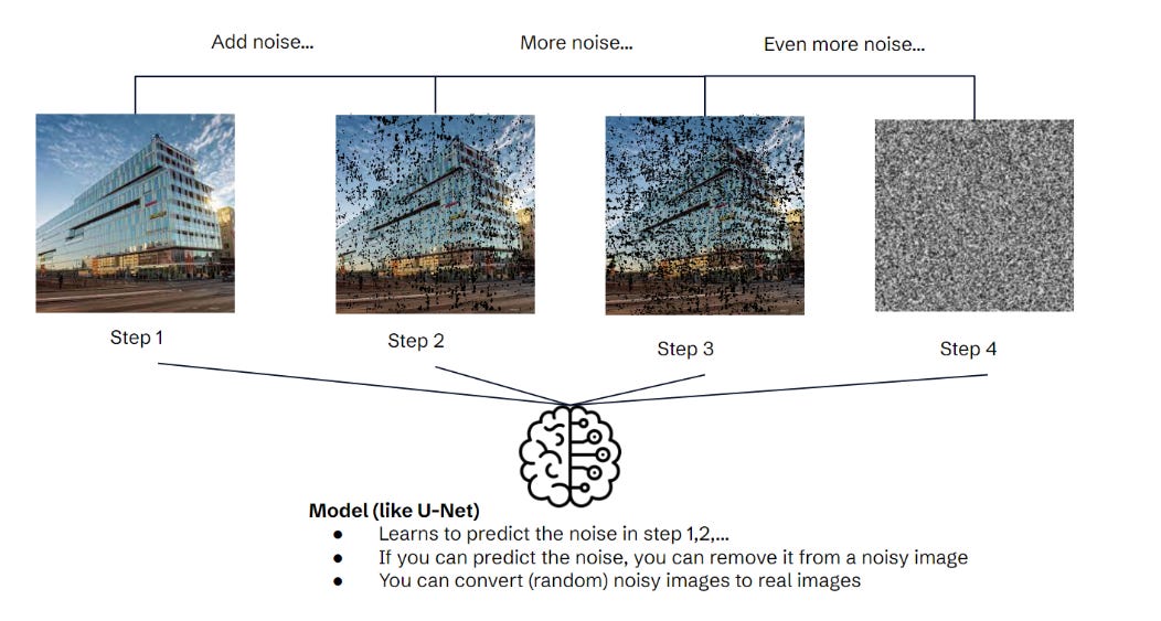
In the training phase, you create noisy images by iteratively adding more noise. Then, you train a model to predict the noise based on the image and the timestep. For example, the model can predict the noise at timestep 3 for an image of Schibsted’s Stockholm office. You can now use this model to create new images. Just generate some noise and remove it from the current image step-by-step - voilà a new image emerges. You might now wonder how to ask for a specific image, like a car or a cat. You can’t. We just learned that you only input noise and the model generates whatever.. Unconditional image generation creates random images of concepts it was trained on. To produce images from certain concepts, you need a conditional generation model like Stable Diffusion. [Paper]
Stable Diffusion
Stable Diffusion is one of the most popular image generation models and was originally released in August 2022. Its architecture is called the “latent diffusion model”. It works like this:
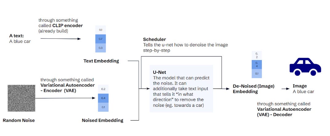
Input: You can input text and random noise. The latter is generated automatically, so an end-user doesn't need to care about that.
Compression: Both inputs are converted into embeddings. The noise is converted using a Variational Autoencoder (VAE). The idea of an Autoencoder is to create a compression of its input.
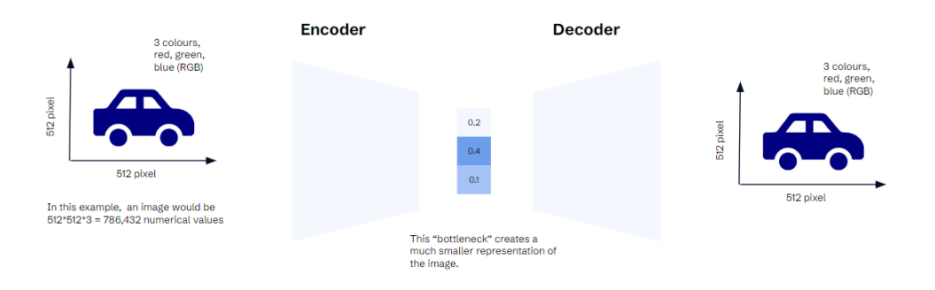
In our example, the car image can be expressed as ~786k numerical values (height in pixel x width in pixel x 3 values for each colour). To compress that image, you use a neural network with two parts. An encoder reduces the number of values. A decoder recreates the same image from those intermediate representations (aka embeddings). These intermediate representations come in handy for Stable Diffusion. Instead of doing operations on 768k values, you can use the much smaller embeddings. The “variational” in VAE comes from adding a bit of controlled randomness between the encoder and decoder, but it does not matter here. To convert the text, Stable Diffusion uses a pre-trained CLIP encoder. It creates embeddings that capture the semantic information but in a lower dimensionality than the original data.
Removing the noise: Once we have (noisy) image and text embeddings, we use the U-Net (same as in unguided diffusion above) to denoise the image embedding. However, there is an important change - the U-Net also takes the text embedding as input. Supported by a scheduler, the U-Net removes the noise of the image embedding step-by-step until we have a denoised image embedding.
Output: We use the VAE decoder to convert the denoised image embedding into a proper image.
Training Stable Diffusion
To combine all those elements, we can train a Stable Diffusion model in three steps:
Get the CLIP (Text) Encoder - This encoder is already pre-trained, so we don’t need to train it ourselves.
Train a Variational Autoencoder (VAE) - the VAE is trained unsupervised since it tries to reconstruct its input. So, we only need a set of images.
Train the U-Net - since CLIP Encoder and VAE Encoder & Decoder were trained in 1) and 2), we can keep them frozen in the training process. We need to have a dataset with prompts (text), random noise, and output images.
Fine-Tuning with Dreambooth & LoRA
Luckily, we don’t have to train the Stable Diffusion model from scratch. If we want to teach it new things, we have to fine-tune it.
One of the most popular methods for fine-tuning is Dreambooth. Its general idea is to teach the model a new concept from only a few images. It does that by refining the U-Net, while the rest of the model is frozen. The authors figured out that the most efficient way is to use the prompt of the form “a [identifier] [class]”, for example, “an sks dog”. In this way “dog” utilizes an already learned concept, while “sks'' creates a new identifier for that particular dog.
One issue with Dreambooth is its requirement for the full U-Net to be trained, demanding substantial memory and computational resources. Here LoRA becomes relevant. LoRA is an adapter-based method, which involves adding a few additional parameters to the model. At first glance, this approach may seem counterintuitive - why would adding more parameters decrease memory consumption? The reason is that only these new parameters are trained, while the old ones remain frozen. As a result, training fewer new parameters means reduced memory requirements for gradients and optimizer states.
Another method for fine-tuning is called Textual Inversion. The idea is to add a new token to the text (CLIP) embeddings and train this embedding to generate our training images. The rest of the model is frozen. The disadvantage of this method is that it can only reproduce what the model already learned in pre-training, since the diffuser/U-Net is not trained.
In practice, a hybrid approach is most common. In the first phase of the training you create new tokens and try to get as close as possible to the training data. Then you apply Dreambooth to nudge those new tokens towards the new concept.
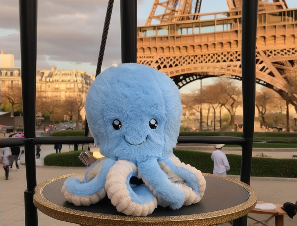
Experimenting with “Otto”
Training
In my experiment, I wanted to train a model to generate images of Otto, one of our mascots. The implementation used hugging face diffusers and one of their pre-build training scripts. I used the default parameters except for the following:
instance_prompt “a blue plush octopus” - The prompt to identify my images. It followed the original Dreambooth paper by defining the class “blue plush octopus” and the instance “”. I played a bit with changing the wording, but it does not seem to have an impact.
gradient_checkpointing - Instead of saving all the immediate activations, only certain checkpoints are retained. Makes training slower, since they need to be re-computed, but saves a lot of memory.
mixed_precision="fp16" - Let you keep parameters, gradients, and activations in float16 and thereby reduce memory.
Train_text_encoder_li - I turned on textual inversion training for the first half of the training, and the second half switched to Dreambooth
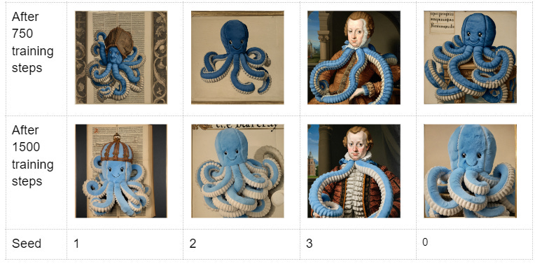
I trained it on an L4 GPU on GCP (24 GB memory). A fine-tuning run with 15 images and 1,500 steps took 3-4 hrs. In the first training experiment, I just ran 1500 steps and compared the intermediate results:
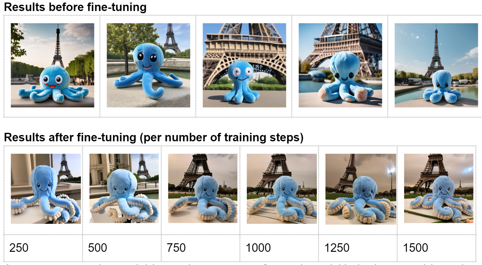
As you can see, the model learned to re-create Otto quite quickly in the textual inversion phase. That could indicate that he has been in the pre-training data already, which could be realistic since he is a quite popular toy. Also, the prompt “blue plush octopus” is quite specific.
Generation
Retrieving a good image is a much more brittle process than training the model. Essentially, you can modify the following hyperparameter:
Prompt: What do you want to ask the model? What order? What level of detail?
Seed: Since the diffusion model uses “random” noise, the output differs for every generation. By keeping the seed fixed, this randomness is removed from the model. This seemed to be the most impactful parameter for me.
Guidance Scale: A parameter that determines how much the model is directed by the text prompt (higher) and how creative it can be (lower).
Denoising steps: Determines how many de-noising iterations the U-Net does. The more, the better the quality. On the other hand, more steps also increase the required time.
So, I conducted a few experiments to find the optimal combination:
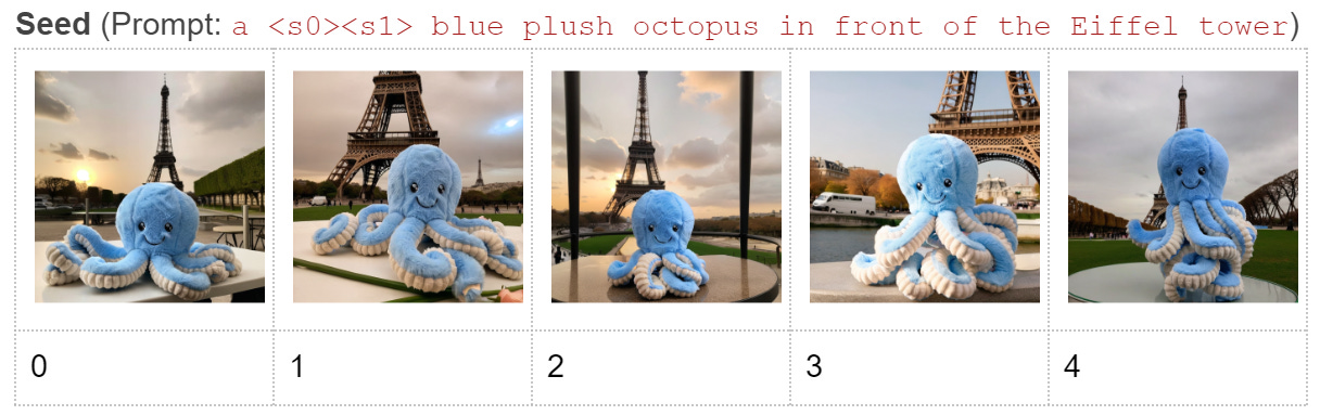
I used a torch generator to fix the seed (code below) and got different outcomes for each seed.
generator = torch.Generator(device="cuda").manual_seed(i) img = model(prompt, generator=generator, num_inference_steps=50, guidance_scale=7.5).images[0]
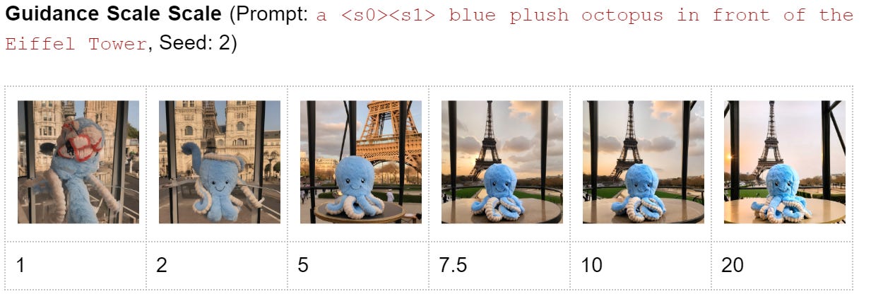
The results between 5 and 10 looked good to me, so I continued with 7.5.
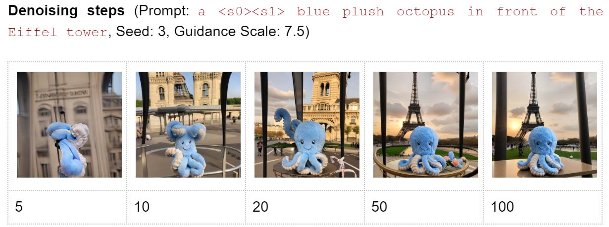
More denoising steps provided better results, but they also took more time. So, I select 50 golden middle ground.
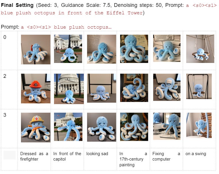
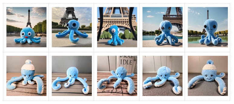
I was happy with the overall results, but interestingly we observed two cases where the model failed:
Generate a 17th-century painting of him - he would always sit in front of the painting instead of being its subject.
Make Otto look sad - he just always kept his happy face.
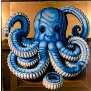
Concept Transfer: A 17th century painting of…
In my initial experiments, Otto always looked very plushy and just not integrated with the 17th-century painting. It was easy to fit him into places or dress him differently, but he would not as well merge with entirely new concepts.
To my surprise, loading the training checkpoint from 750 improved image generation. I suspect that there was some overfitting at play.
Finally, I managed to get a single good image of him. I removed “plush” from the prompt and increased the guidance scale to 15. I suspect that removing “plush” eased some of the over fittings, while the high guidance scale forced the model to value “sticking to the prompt” higher than “high quality.”
Extrapolation: A sad plush octopus
Generating a sad octopus was impossible. Even in the original model, it was not easy to make it smile. After fine-tuning on an ever-smiling Otto, all hope was gone. I tried different configurations, but he would only smile. I partially attribute this to his training data (only smiles) but also the problems with generalization (like in the painting).
Learnings
Summarising all of this, these were my main learnings:
Training the models is cheap and easy: In 3-4 hours you can fine-tune your Stable Diffusion model. The real cost lies in the time you need to figure out the right settings.
Training is very brittle: The output is very sensitive to the parameters. There are few best practices, so you need to experiment a lot.
Power is in the prompt: The largest improvements I got when modifying the generation process (especially the prompt). Tweaking the training could have been more impactful.
Overfitting and generalization: The problems with the 17th-century painting and sad face showed that the model learns Otto as an entity rather than a concept. There are certain things to prevent overfitting, like early stopping or removing keywords from the prompt, but that does not necessarily make generalization better.
Luckily, my employer Schibsted is very supportive of learning and I got the time to work on the article as part of one of our projects.
If you want to connect, please subscribe or add me on LinkedIn.